Shrimp production simulation models
A powerful tool to increase farming efficiency

The evolution of computers has led to the development of mathematical models to help solve complex problems. The most common models are electronic spreadsheets (e.g., Microsoft Excel) used for business applications. These compile a series of cost and revenue relationships to allow examination of the behavior of business as a whole. This helps managers choose business scenarios that maximize overall profitability.
The same modeling concept is being applied to shrimp ponds to characterize the physical, biological, and chemical processes in these complex ecosystems. This helps managers identify interventions that maximize profitability without environmental and social impacts.To deal with the enormous complexity of multiple, interacting, and constantly changing factors within shrimp ponds, we developed a simulation-type model (see inset for a brief description of the various types of models).
Development of simulation model
Our simulation model was developed to represent low water- exchange, intensive shrimp production systems that receive dry feed and have a strong microbial community of bacteria and phytoplankton. The model has a biological and an economic compartment (see Figs. below). The model is mechanistic and deterministic.
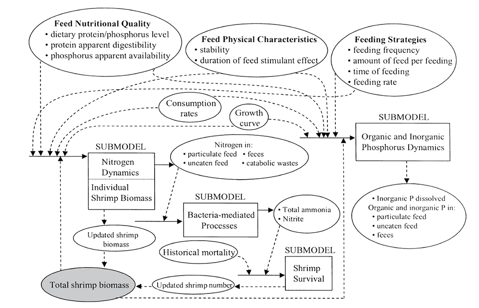
Biological compartment
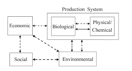
environmental, and social factors limit the application of scientific research to predict behavior of aquaculture production systems. Dotted lines represent information transfer; solid lines represent material transfer.
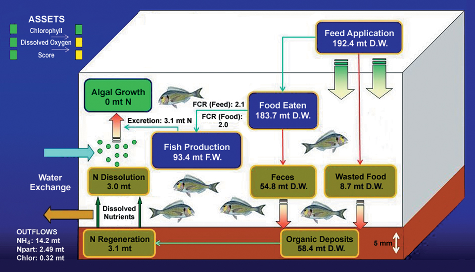
The biological compartment deals with the daily addition of nitrogen and phosphorus to the culture system as feed. It estimates rates of feed consumption and metabolism by shrimp. It also represents loss of the components as uneaten feed (whole pellets and particles), feces, nitrogen excretion as ammonia, and inorganic dissolved phosphorus.
Nitrogen incorporated by shrimp determines shrimp growth. Nitrogen and phosphorus in uneaten feed and feces are used by heterotrophic bacteria, which may regenerate ammonia, depending on carbon to nitrogen ratios (C:N) of these organic substrates. Nitrogen excreted as ammonia is utilized by heterotrophs and nitrifying bacteria. The activity of nitrifying bacteria determines ammonia and nitrite levels, which affect shrimp survival.
In this manner, the model can be used to examine the effects of any combination of the following parameters at any point in time during the culture cycle:
- feeding rate
- feeding frequency
- time of feeding
- amount of feed per feeding
- dietary protein level
- protein digestibility
- duration of feed stimulant effect
- feed stability
- dietary organic and inorganic phosphorus levels
- organic and inorganic phosphorus availability
- inorganic phosphorus leaching rate
- initial shrimp number
- initial shrimp weight
- initial ammonia, nitrite and nitrate concentrations.
These factors affect:
- shrimp growth
- shrimp survival (due to toxic levels of ammonia and nitrite and site-specific mortality)
- total inorganic phosphorus concentration
- organic phosphorus load
- ammonia, nitrite and nitrate concentrations
- organic nitrogen load
The model also predicts water exchange required with a mortality warning display.
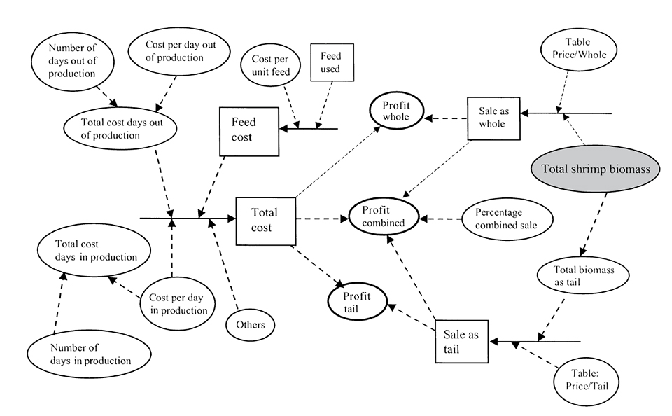
Economic compartment
The economic compartment predicts daily operating cost and total operating cost, and allows the comparison of profitability based on market preference (tail head-on, or a combination of both). Shrimp growth and survival predicted by the biological compartment is used by the economic submodel to update cost and profitability.
Model performance
Model results were compared to unpublished and published research results from the Texas A&M Shrimp Mariculture Project (Texas, USA), the Waddell Mariculture Center (South Carolina, USA), and the Oceanic Institute (Hawaii, USA). This model predicts shrimp growth and survival in these types of systems with a 90 percent confidence level. Efforts to compare the model predictions to production and water-quality results from commercial intensive operations are currently under way.
One of the critical areas identified by the model that needs much consideration is the determination of the initial bacterial and phytoplankton community within the system, because of the important role they play in recycling nutrients. To more accurately represent bacteria and phytoplankton dynamics, a carbon-cycling submodel is currently under construction to be added to the biological compartment described above. This is another advantage of this type of model. It has the flexibility to accept additional components in successive steps, while working and generating results with the current model.
Conclusion
As shrimp-farming systems intensify, there is a growing need for powerful tools to predict the economic, social and environmental impact of prospective interventions. Simulation models are a powerful tool, because they allow the combination of any number of factors that would be impossible to examine experimentally at one time, due to both cost and time limitations.
Simulation models can be used to predict the most critical management factors and levels, thus optimizing time and resources. They also allow representation of the effects of random situations, such as mass mortalities and low market prices, on general production factors. This allows managers to plan ahead and develop appropriate risk-management practices.
Models are…
Although models developed for aquaculture can be classified in several ways, it is instructive to broadly categorize them based on the approach used to construct them, or on their structure. Based on their construction, models can be biologic, biophysic, economic, or bioeconomic. Based on their structure, models can be static or dynamic, empirical or mechanistic, deterministic or stochastic, and simulation or analytical.
Static / synamic
Static models describe relationships that do not change with time, such as some types of regressions. Dynamic models describe a time-varying relationship, such as regressions that include time as a variable.
Empirical / mechanistic
Empirical or correlative models are developed to describe a set of relationships without regard for the appropriate representation of processes that operate in the real system (e.g., a model predicting metabolic rate solely as a function of body size). Mechanistic or explanatory models are developed to represent the causal mechanisms underlying system behavior (e.g., a model representing the metabolic rate as a function of body size, level of activity and environmental temperature).
Deterministic / stochastic
A model is deterministic if it contains only non-random variables (e.g., a model relating energy requirement to ambient temperature). While, stochastic models contain random variables (e.g., the above model in which ambient temperature is represented as a random variable within a temperature range). Thus, stochastic predictions under a set of conditions are not always exactly the same.)
Analytical / simulation
Models such as exponential population growth, which can be solved in closed form mathematically, are analytical. Simulation models do not have general analytical solutions. Therefore, they must be solved numerically using a specific set of arithmetic operations for each particular situation. An example is a population growth model as response to availability of resources, diseases, and environmental changes.
This model classification is not exclusive and may be combined with other model types to accurately describe a system. For example, we can build a simulation model that changes with time and does not have analytical solutions to represent biological processes. However, it can also be mechanistic (explains internal dynamics) and deterministic (does not have random variables).
Simulation models for complex systems
In most cases, when interest is centered on complex systems, simulation models are the most appropriate tools to use. Complex systems refer to those with many closely related components. Also, the dynamics of complex systems cannot be represented statistically as average tendencies, because interrelationships of components cause non-random behavior (i.e., fish biomass affects feed consumption today, which will again affect the biomass tomorrow, and so on).
(Editor’s Note: This article was originally published in the February 2001 print edition of the Global Aquaculture Advocate.)
Now that you've reached the end of the article ...
… please consider supporting GSA’s mission to advance responsible seafood practices through education, advocacy and third-party assurances. The Advocate aims to document the evolution of responsible seafood practices and share the expansive knowledge of our vast network of contributors.
By becoming a Global Seafood Alliance member, you’re ensuring that all of the pre-competitive work we do through member benefits, resources and events can continue. Individual membership costs just $50 a year.
Not a GSA member? Join us.
Authors
-

System Analysis Specialist and Consultant
Ciudadela Los Ceibos
Avenida Segunda #321 y Calle Décima
Guayaquil, Ecuador -
Director of Nutrition and Research
Empacadora Nacional
Guayaquil, Ecuador
Related Posts
Innovation & Investment
Bio-economic modeling for improving aquaculture performance
Experience in China, the world’s largest tilapia farming country, is used to develop and calibrate a bio-economic model of intensive tilapia pond culture. It is used to simulate the impacts of climate, technical and/or economic factors on farming.
Health & Welfare
Computer modeling helps grow fish
For farmers, computer modeling helps analyze crop production and environmental effects. For managers, it assists with carrying capacity assessments and licensing issues.
Health & Welfare
Genome editing potential to improve aquaculture breeding, production, Part 2
Genome editing can contribute to sustainable aquaculture production in terms of disease resistance and sterility to prevent interbreeding with wild stocks.
Health & Welfare
Innovative techniques achieve more cost-efficient salmon selective breeding
Successful non-invasive predictions of pigment and fat levels in whole salmon were demonstrated by the authors using visible and near infrared spectroscopy to study how these traits vary genetically during growth.